Reconfiguring the Base Network

I can be contacted at E-mail address:-

It is a good plan to first explore the working ‘Base’ Network as generated by the installer to become familiar with the features and functions of Radio Mobile by using the provided Base, Mobile and Hand Held units located on the map area.

1 - Relocating the Map:

First it is necessary to have an Internet connection available to download the additional SRTM elevation data required by a new location.

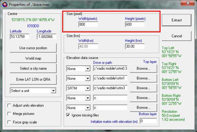
Open the ‘Map properties’ pane using function key ‘F8’ or the toolbar icon and you will see the on-screen map dimensions are set at the top of the pane in screen pixels:

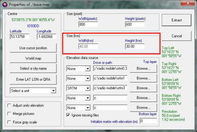
The actual ground area shown is defined as below where only the map ‘Height’ in km can be changed with the ‘Width’ being calculated from the pixel settings above.

The new Map centre location can be defined in a number of ways as shown in the area below.

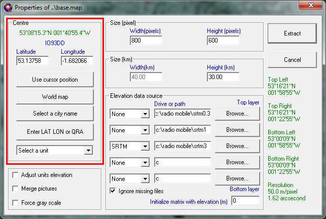
First, ‘Use cursor position’ is useful where only a small adjustment of the on-screen map centre is required. This function can quickly be enabled by a ‘double left click’ on the map location which will open the Map properties pane with the cursor coordinates entered.

Second, for large movements the World map can be selected using ‘View/World map’ or ‘Ctrl+W’ and the cursor placed at the required location for the map centre.

Third, Google Earth can be used as the source of the required coordinates to enter when using the ‘Enter LAT LON or QRA’ button. The picture below shows the approximate area of my Base map as viewed in Google Earth.

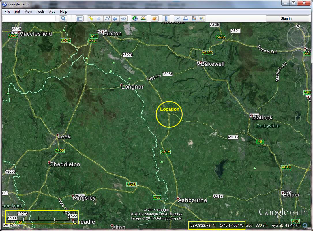
Placing the screen cursor at the road junction shown in the yellow circle centre screen allows the cursor coordinates to be recorded from the lower right ‘Coordinates’ area.

The required map size can also be approximated by using the lower left ‘Scale’ or Google Earth measurement tool for entry into the Map properties pane.

Finally the ‘Select a city name’ button can be used where your nearest major city can be selected. This was left to last option as the Merge function is required to confirm the actual area location. You can either type the first few letters of the city name or use the scroll keys to navigate the listing:

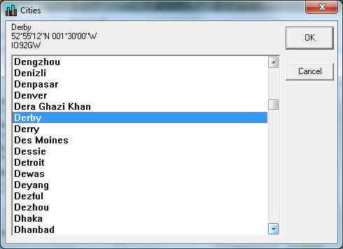
You will notice that the city Latitude and Longitude are shown at the top of the pane, and a click on the ‘OK’ button enters these into the Map properties ‘Centre’ location box.

Regardless of the method used, clicking on the ‘Extract’ button initiates the download of new SRTM data from a selected mirror site and the data is deposited into the SRTM3 folder for use. The new elevation map will then be drawn.

At this stage it is impossible to confirm where the map is actually located and its coverage extent, but by downloading a Road map of the area you can check the location if you have agreed to the terms and conditions in, and modified, the Map_Link.txt file during installation. If Map_Link.txt hasn’t been modified when offered by the installer, the lower three internet download sources will not appear on the Merge pane below.

To download a Road map you need to use the Merge function key ‘F7’, the toolbar icon or ‘Edit/Merge pictures’ from the toolbar.

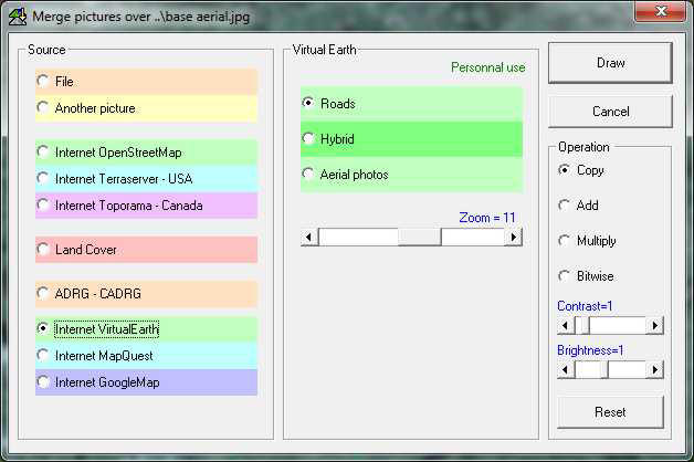
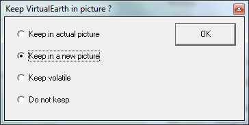
The pane above shows ‘Internet Virtual Earth’ as the data source with ‘Road’ maps selected and with the ‘Operation’ set as ‘Copy’. Clicking the ‘Draw’ button then initiates the download of the road map data for the exact map area, and a coloured picture will appear accompanied by the selection pane below. If you ‘Keep the picture in a New picture’ as shown it allows you to decide if you want to permanently save it or discard later when closing the program.

Assuming that you now have a suitable map area you can use this new picture to add the road detail to your elevation map if you wish as can be seen on my Base Network map. First convert the picture to Greyscale using ‘Edit/Force greyscale’ and decide if you wish to have a new picture or overwrite the existing coloured picture. Grey scale is better as this does not confuse the colours of the elevation map and the picture could also be used as the canvas for coverage plots later.

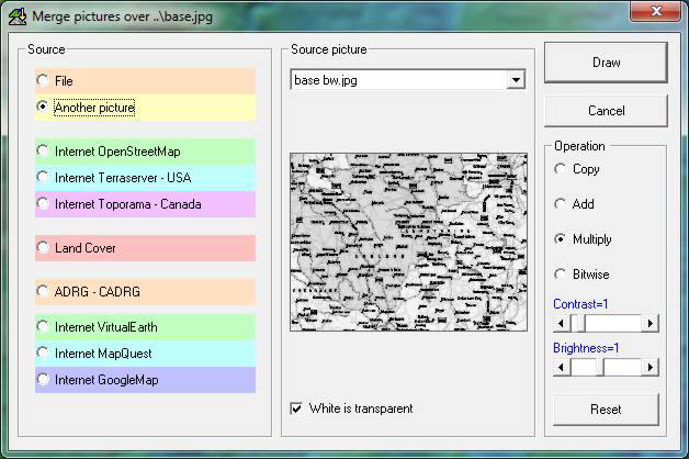
Next Open your Elevation map picture and once again use ‘F7’ for a Merge, but in this case select ‘Another picture’ as the ‘Source’ and after selecting the greyscale picture from the drop down list, use the ‘Multiply’ operation to lay the road network over the elevation map. If suitable, you can then keep this in the picture and save once more. Check that ‘White is transparent’ has been selected on the merge pane to ensure that the elevation data colours aren’t modified.

At this stage you can cycle through your open pictures using ‘Ctrl+Tab’ keys or ‘Ctrl+shift+Tab’ for the reverse direction and close all my Base Network pictures. It is also worthwhile to save your data in a New named folder in the program ‘Networks folder’ – there are three folders present, one named ‘Base network’ plus two other empty ones called ‘Network 2’ and ‘Network 3’. Rename one of these empty folders to your network name and using ‘File/Save network as’ navigate this named folder, open it and then Save your Network with your own name. Next run down the ‘File’ drop down list and ‘Save Map as’, ‘Save picture as’ for all pictures including your elevation map. It is also worthwhile to ‘Save Network as’ using your own name in the same folder so that later you can just save the network to the same folder after any modifications have been made.

2 – Relocating and modifying Unit names:

The installed Base Network has three units specified, but these are placed on the original map area coordinates so need to be moved to their new locations before modification to your own requirements. First click on a suitable location on your new map and open the ‘Unit properties’ pane using ‘Ctrl+U’ or by using the icon on the taskbar.

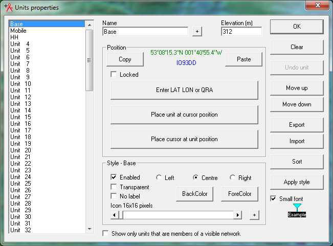
Next select a Unit and click on the ‘Place unit at cursor position’ button. This needs to be repeated for all three units and then it would be wise to ‘File/Save network as’ after navigating to your new folder to make sure that you have your changes saved.

This is the pane where you can also modify the Unit names, add new ones, change their screen icons and their label formats as required.

3 – Modifying Network Parameters:

The Network properties pane (accessed using the icon, ‘File/Network properties’ or ‘Ctrl+N’) below controls all the parameters utilised by Radio Mobile for its calculations. The pane will open and show the Parameters tab:

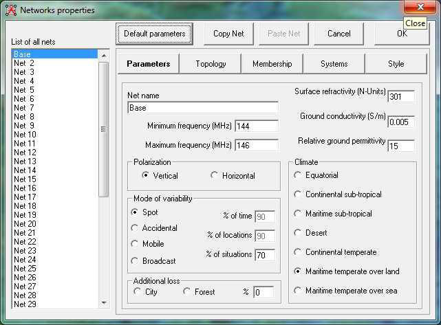
This is the pane where all the climate, polarisation, frequencies and network name can be changed or adjusted.

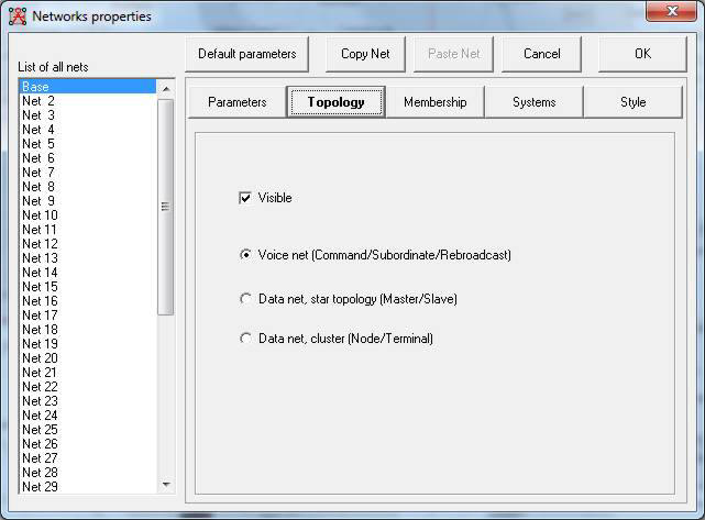
With the second ‘Topology’ tab seen below, the actual type of network can be selected, this has a bearing on the way that radio links over the map area are displayed.

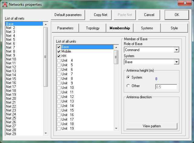
The next Tab ‘Membership’ shows the members allocated to the Network and their ‘Roles’ as Command, Subordinate or Rebroadcast functions. The separate Unit Radio Operating ‘Systems’ are also allocated and specific Unit antenna heights adjusted from their ‘System’ settings if required.

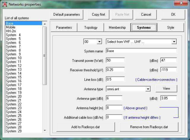
The ‘System’ tab gives a set of radio configurations which define the complete radio setup for a location. Each radio Unit is allocated to a Radio Operating ‘System’ as can be seen below. Thus many identical units can be allocated to a specific Radio Operating ‘System’, but each radio unit can only have one.

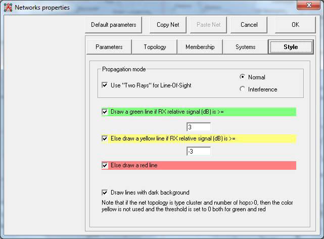
The final tab ‘Style’ shown below first controls the use of the ‘Two ray’ method for the ‘Line Of Sight’ path propagation mode. This can be set as ‘Normal’ or ‘Interference’ and can also be disabled if required.

Below this area are the settings for the ‘Style’ of radio Link displays – the limits for the colours of radio links shown on the plots can be set in dB’s relative to the receiver threshold. Thus with the default settings shown, any link where the signal level is +/-3dB from the receiver threshold will be shown in yellow. Higher signal level links are shown as green, and lower levels as red.

Where the two level settings are made equal the yellow colour is suppressed so this may be used for Go/No-go plots.

Combined Cartesian plots have the feature where ‘Style’ plots can be performed using the settings above, and if a ‘Route Radio Coverage’ plot is performed the Style colours are displayed on the Route plot indicating the signal levels calculated.

4 – Changing the downloaded SRTM data resolution:

The Base network settings have been selected to use the 3 arc-second SRTM data with a resolution of approximately 90m for two reasons. First the 1 arc-second data has only recently become available, and second as a single SRTM tile is provided with the installer and the 2.5MB size of a 3 arc-second tile reduces the download size compared with the use of a 25MB 1 arc-second tile.

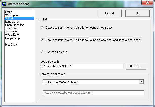
To modify the program dataset to 1 arc-second requires two changes. The first change is on the ‘Internet Options’ pane accessed by ‘Options/Internet’ and selecting the SRTM tab as shown below. Here the local path has been set to the SRTM1 folder, and also the ‘Internet ftp directory’ has been changed to ‘SRTM-1 arc-second’ data.

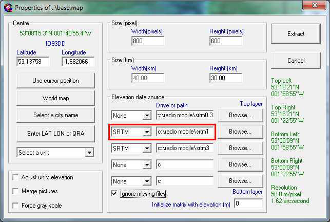
Next the Map properties pane has to have the 1 arc-second data folder enabled as can be seen in the pane below where the red box shows that the SRTM1 folder has been enabled for map access. Data is accessed from the top layer down when data becomes unavailable.

A click on ‘Extract’ will now cause the higher resolution data to downloaded from the internet and a new elevation map to be drawn.

5 – Changing the number of records to be used by the propagation model:

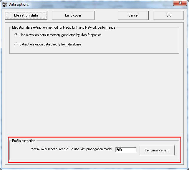
Examine the ‘Data Options’ pane below by using ‘Options/Elevation data’. In the lower Profile extraction area it shows that the number of records to be used by the model has been set to ‘500’ by the installer.

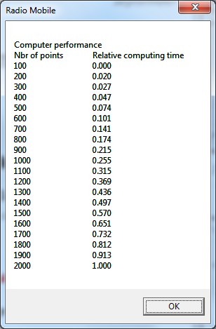
This number can be increased to a maximum of 2,000 thus increasing the number of data point calculations but also increasing the computational time. Before changing this value it is worthwhile checking your computer performance by clicking on the ‘Performance test‘ button which then generates the pane showing the relative time penalty incurred by the change in number of records. The relative computing time will affect all coverage plots performed.

Also remember that any program computation can be ‘paused’ by use of the keyboard Space bar if necessary, with a warning appearing on the bottom data area of the program pane.

6 – Selecting optimum settings to obtain highest plot accuracy:

It is important to note that the elevation map pixel resolution has to match the elevation data resolution to obtain the most accurate coverage plots. To this end on the ‘Elevation data’ tab shown above, first use ‘Elevation data in memory’ with the maximum number of records to use set to 2000.

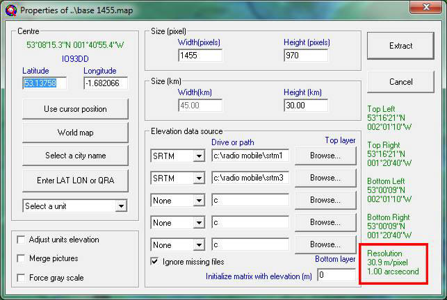
On the ‘Base 1455’ map properties pane above you can see that the pixel resolution has been adjusted to become 1.00 arc-second by changing the map size in pixels from the 800x600 screen size of the installer ‘Base’ map.

When using 2000 records the maximum map size would be 4000x4000 pixels, and thus the circumference of the plot would then be 2xπx2000 = 12566 pixels. This would then require an azimuth step of (360/12566) = 0.0286 degrees for the plot, (or when using 1000 records 0.057 degrees step size) to make pixel steps at the plot circumference.

Selecting a map size of over 2000x2000 pixels does raise a warning on the map pane as operation beyond this size is governed by performance of the computer including RAM installed and the video card memory available.

With Combined Cartesian plots use a radial range to avoid stretching the calculations into the map corners – these plots are much slower than the polar plot shown above. There are additional functions available from Combined Cartesian plots.

Don’t forget to save any program changes made, there is a reminder before the program closes!