Best Unit for coverage
I can be contacted at E-mail address:-
![]()
Best Unit for coverageI can be contacted at E-mail address:-
|
|
|
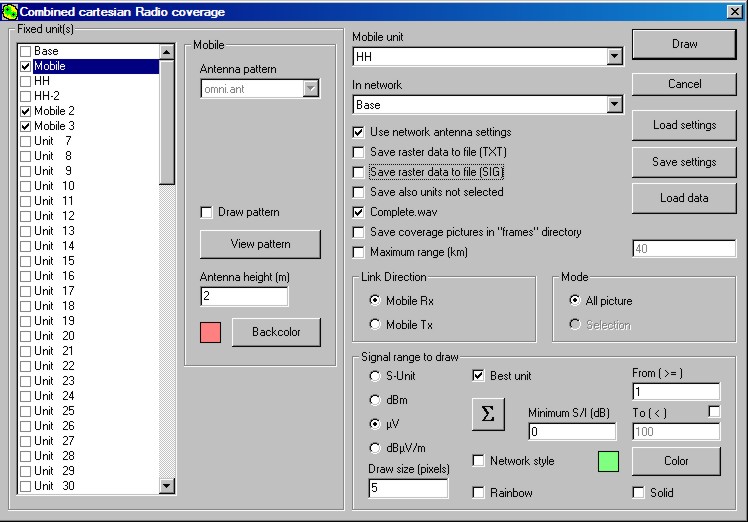
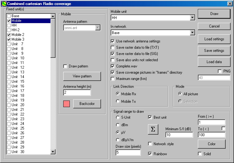
As an alternative to the Signal strength displays as in 'Multiple Unit' Coverage, where it is required to find the 'Best Unit' to provide the maximum signal at a location, return to the greyscale road map, and re-open the Cartesian Coverage pane. In this case check the 'Best Unit' box as shown. Selecting a fixed Unit will then allow the Background Colour of the Unit Label to be changed - this colour will be used to identify the 'Best Unit' on the resulting plots.
By using the 'Save raster data to file (SIG)' option, a signal level matrix (*.sig) file will be generated during the plotting process. This file then provides a calculated signal level readout at the cursor location for the whole plot, and will be saved with any coverage plot.
The Best Unit check box opens another control window 'Minimum S/I[dB]'. This window enables a Signal level to Interference margin in dB to be set for the Best Unit plot thus allowing the co-channel performance of the mobile unit to be taken into account for the plots. For the following plots this level has been set to 0dB so that they only show the Best Unit signal level at a location. The effect of changing this margin can be seen Here.
Pressing the Draw button will, with the settings below, cause three sequential individual plots to be performed for the coverage of the Mobile, Mobile 2 and Mobile 3 to be performed, followed by a final displayed plot showing the best unit for each location on the map. In this case, as the Raster data isn't saved to file, only the final Best coverage areas will be shown, and no signal level legend will be shown. (As Picture2 below).
If the signal level legend is required, first perform a quick Polar plot using the signal range options above, and then discard this without saving. This action generates the 'last legend' required for the following coverage plots.
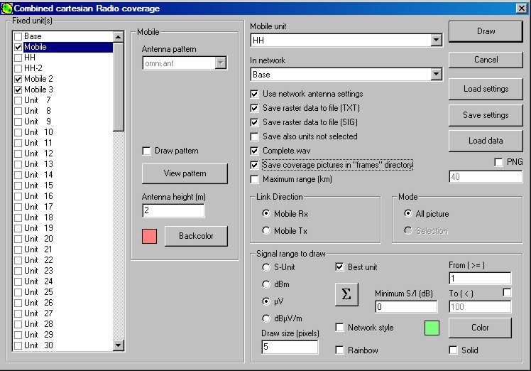
Next select both the 'Save raster data to file', (TXT - and SIG if required) and 'Save coverage pictures in 'Frames' directory' as shown.
Selecting the PNG box on the 'Save coverage pictures' line causes the saved pictures to be generated in PNG format rather than bmp. The advantage of this is that the picture had a transparent white background allowing it to be exported into Google Earth - if present on your computer - by a click on its kml file.
On pressing 'Draw', the program will generate a numbered 'Frames' directory your network folder to contain the individual coverage plots. Each Unit individual coverage pattern will be plotted and stored along with the combined coverage plot, followed by the window below showing the Best Unit for cover at any point on the picture, as indicated by the Unit Background colour.
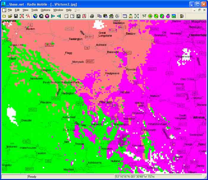
The separate coverage pictures can then be opened by looking in the Base Network folder for the 'frames001' folder. This holds files cov0001-cov0003 corresponding to the three individual mobile plots, plus the combined coverage files. Open the first plot, then using 'Edit/Redraw last Legend', and 'Keep in picture' will provide the reference signal legend on the plot if required. This can then be repeated for the other two plots, keeping all the plots open.
Finally, placing the cursor at a location of interest on the Best Unit plot allows the saved signal strength coverage pictures to be displayed to obtain the actual signal levels for each unit at that point.
If the 'SIG' file option has been invoked, the actual signal level at any cursor location can be recalled negating the addition of the picture legend. On changing plot windows (using Ctrl-Tab or Ctrl-shift-Tab), the associated SIG matrix file has been registered and the signal level at the same cursor position will be displayed.
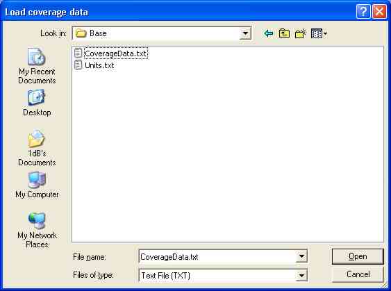
Using previous coverage data: As an alternative to the above, you could use the Data generated and saved in a previous Multiple Unit coverage plot by clicking on the 'Load Data' button.
The program will prompt for the location of the previously saved Coverage file (as shown on the Multiple Unit Coverage page) which can then be loaded.
and produces the following window showing the Best Unit for cover at any point on the picture, as indicated by the Unit Background colour. Placing the cursor at a location of interest then allows the previous signal strength pictures to be displayed to obtain the actual signal levels at that point.
Note that if the 'Best Unit' box is checked, and the Draw button pressed, the separate signal coverage plots will be performed, and the pictures saved in the Frames directory - there will be a 'Combined Signal Coverage' plot also available. Loading the coverage data as above but without the 'Best Unit' box checked will produce a combined coverage plot - but with a dB legend displayed. So it is worthwhile performing a 'Rainbow' plot first to obtain this.
The above process can also be carried out on a zoomed area of the map for a 'Detailed Area Coverage' plot.
Effect of Signal to Interference (S/I [dB] margin setting.
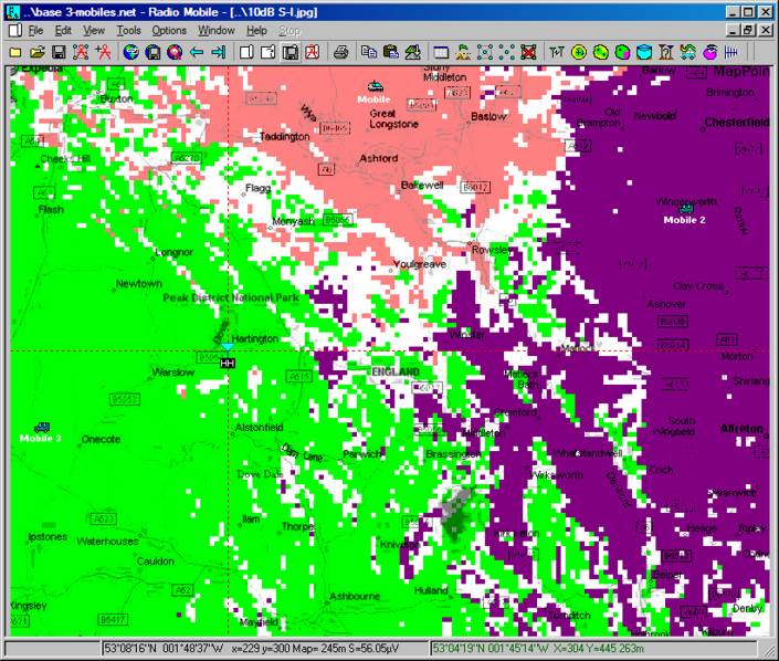
The next pane has had the S/I margin changed to 10dB, the SIGnal files have been selected and saved in a Frames directory to use later. Note that in the 'Signal range to draw', a signal level range of 1µV to 100µV has been entered, but the 'To [<]' box has been cleared allowing the full signal range to be utilised.
Pressing Draw then causes the sequential signal coverage plots to be performed for the three Mobile units, followed by the calculation of the Combined coverage plot shown below. 'Mobile 1' in the light Red area, 'Mobile 2' in the Purple area and 'Mobile 3' in the Green area.
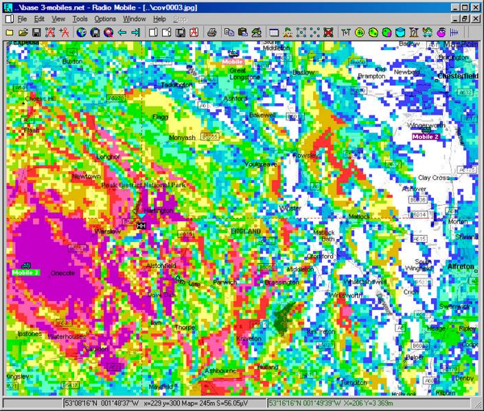
The HH unit has been placed near Hartington, and the cursor placed at its location with a signal strength of 56.05µV shown at this Green location. Comparing this plot with the initial 0dB coverage plot it can be seen that there are White areas between the colours showing that the 10dB signal margin hasn't been achieved - or the received signals are too low for communication.
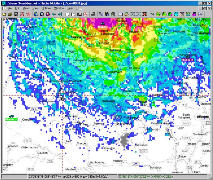
Opening the Coverage plot for 'Mobile 1' shown below, the reported signal at the same cursor location at the HH is shown as 1.00µV.
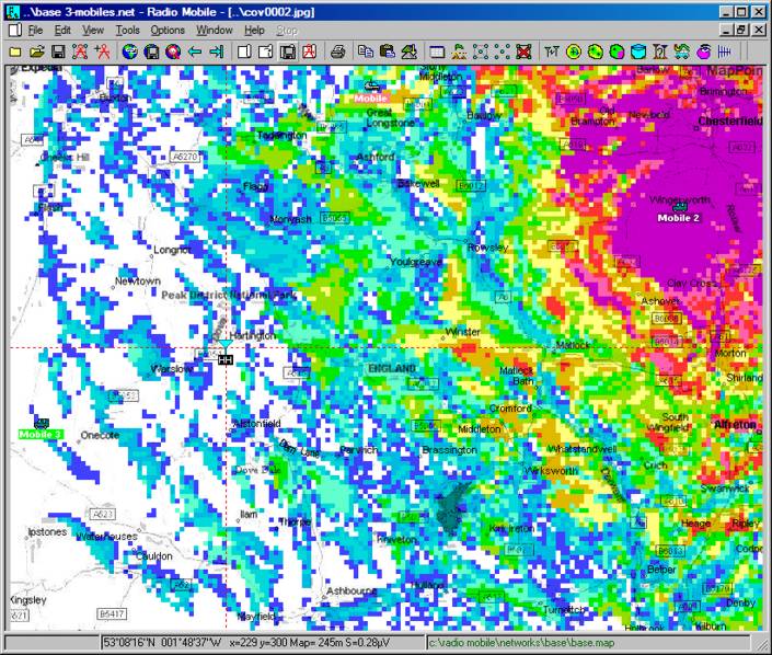
Next opening the coverage plot for 'Mobile 2' and with the cursor at the HH unit location, a signal strength of 0.28µV is indicated.
Finally, opening the coverage plot for 'Mobile 3', the cursor signal strength by the HH unit can be seen to be 56.05µV as indicated on the Combined Best Unit Green area.
Thus it can be seen that at the cursor location 'Mobile 1' produced a marginal signal level, 'Mobile 2' was below receiver threshold and 'Mobile 3' produced the working system. Exploration of the white zones showed the signals were either within the 10dB S/I margin set, or below the receiver signal threshold.
But also see the Multiple Unit Coverage page!
This page is available in .pdf format here
Please keep checking back for updates/additions.
© Copyright G3TVU 26th October 2017
|